External Cluster Validity Measures

In this section, we review the external cluster validity scores that are implemented in the genieclust package for Python and R [20] and discussed in detail in [24].

Let \(\mathbf{y}\) be a label vector representing one of the reference \(k\)-partitions \(\{X_1,\dots,X_k\}\) of a benchmark dataset[1] \(X\), where \(y_i\in\{1,\dots,k\}\) gives the true cluster number (ID) of the \(i\)-th object.

Furthermore, let \(\hat{\mathbf{y}}\) be a label vector encoding another partition, \(\{\hat{X}_1,\dots,\hat{X}_k\}\), which we would like to relate to the reference one, \(\mathbf{y}\). In our context, we assume that \(\hat{\mathbf{y}}\) has been determined by some clustering algorithm.

External cluster validity measures are functions of the form \(I(\mathbf{y}, \hat{\mathbf{y}})\) such that the more similar the two partitions are, the higher the score is. They are normalised so that identical label vectors return the highest similarity score which is equal to 1. Some measures can be adjusted for chance, yielding approximately 0 for random partitions.

Oftentimes, partition similarity scores (e.g., the adjusted Rand index or the normalised mutual information score) are used as \(I\)s. They are symmetric in the sense that \(I(\mathbf{y}, \hat{\mathbf{y}})= I(\hat{\mathbf{y}}, \mathbf{y})\). However, as argued in [24], in our context we do not need this property because the reference label vector \(\mathbf{y}\) is considered fixed. The normalised clustering accuracy is an example of a non-symmetric measure.

Confusion Matrix

Let \(\mathbf{C}\) be the confusion (matching) matrix corresponding to \(\mathbf{y}\) and \(\hat{\mathbf{y}}\), where \(c_{i,j}=\#\{ u: y_u=i\text{ and }\hat{y}_u=j \}\) denotes the number of points in the true cluster \(X_i\) and the predicted cluster \(\hat{X}_j\) with \(i,j\in\{1,\dots,k\}\).

\[\begin{split} \begin{array}{|c||cccc|} \hline {c}_{1,\cdot} & c_{1,1} & c_{1,2} & \cdots & c_{1,k} \\ {c}_{2,\cdot} & c_{2,1} & c_{2,2} & \cdots & c_{2,k} \\ {c}_{3,\cdot} & c_{3,1} & c_{3,2} & \cdots & c_{3,k} \\ \vdots & \vdots & \vdots & \ddots & \vdots \\ {c}_{k,\cdot} & c_{k,1} & c_{k,2} & \cdots & c_{k,k} \\ \hline\hline n & {c}_{\cdot,1} & {c}_{\cdot,2} & \cdots & {c}_{\cdot,k} \\ \hline \end{array} \end{split}\]

It holds \(\sum_{i=1}^k \sum_{j=1}^k c_{i,j} = n\). Moreover, let \({c}_{i,\cdot} = \sum_{j=1}^k c_{i,j} = \#\{ u: y_u=i \}\) denote the number of elements in the reference cluster \(X_i\) and \({c}_{\cdot,j} = \sum_{i=1}^k c_{i,j} = \#\{ u: \hat{y}_u=j \}\) be the number of objects in the predicted cluster \(\hat{X}_j\).

All the measures reviewed here are expressed solely by means of operations on confusion matrices. Therefore, we will be using the notation \(I(\mathbf{y}, \hat{\mathbf{y}})\) and \(I(\mathbf{C})\) interchangeably.

Illustration

The scatterplots depicting the reference and a few example partitions of the wut/x2 dataset are displayed below. We also report the confusion matrices and the values of the validity measures discussed in the sequel.

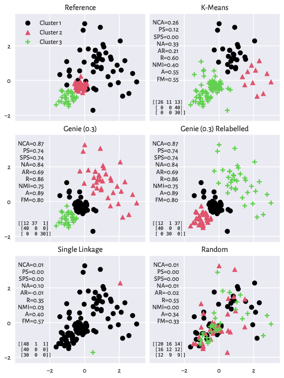
Figure 10: The reference (ground truth) partition and a few predicted clusterings that we relate to it (wut/x2 dataset). Confusion matrices and the values of a few external cluster validity measures are also reported.

Actually, both Genie and the k-means method output some quite reasonable partitions (as we mentioned in an earlier section, there might be many equally valid groupings). Still, here we only want to relate them to the current reference set.

Why Not the Classification Accuracy?

A common mistake is to compute the standard accuracy as known from the evaluation of classification models:

\[ \mathrm{A}_\text{do not use it}^\mathrm{:(}(\mathbf{C}) = \sum_{i=1}^k \frac{c_{i, i}}{n}, \]

which is the proportion of “correctly classified” points. This measure is of no use in clustering, because clusters are defined up to a permutation of the sets’ IDs.

In other words, if the predicted cluster #1 is identical to the reference cluster #3, this should be treated as a perfect match.

Set-Matching Measures

In our context, the predicted clusters need to be matched with the true ones somehow. To do so, we can seek a permutation \(\sigma\) of the set \(\{1,2,\dots,k\}\) which is a solution to (see, e.g., [9]):

\[ \text{maximise}\ \sum_{i=1}^k c_{i,\sigma(i)} \qquad \text{w.r.t. }\sigma. \]

This guarantees that one column is paired with one and only one row in the confusion matrix.

Pivoted and Normalised Accuracy

Optimal pairing leads to what we call here the pivoted accuracy (classification rate [50] or classification accuracy [41]):

\[ \mathrm{A}(\mathbf{C}) = \max_\sigma \frac{1}{n} \sum_{i=1}^k c_{i, \sigma(i)}. \]

It relies on the best matching of the labels in \(\mathbf{y}\) to the labels in \(\mathbf{\hat{y}}\) so as to maximise the standard accuracy. Unfortunately, it is not adjusted for chance. The smallest possible value it can take is \(1/k\). We can thus consider the normalised pivoted accuracy:

\[ \mathrm{NA}(\mathbf{C}) = \displaystyle\max_{\sigma} \frac{1}{k}\displaystyle\sum_{j=1}^k \frac{ c_{\sigma(j),j} - \frac{n}{k^2} }{ \frac{n}{k} -\frac{n}{k^2} }. \]

Implementation: genieclust.compare_partitions.normalized_pivoted_accuracy.

Still, if there are clusters of highly imbalanced sizes, then its value is biased towards the quality of the match in the largest point group.

Normalised Clustering Accuracy

In [24], the normalised for cluster sizes version of NA was proposed. Namely, the normalised clustering accuracy is defined as:

\[ \mathrm{NCA}(\mathbf{C}) = \displaystyle\max_{\sigma} \frac{1}{k}\displaystyle\sum_{j=1}^k \frac{ c_{\sigma(j),j} - \frac{1}{k} c_{\sigma(j),\cdot} }{ c_{\sigma(j),\cdot}-\frac{1}{k} c_{\sigma(j),\cdot} }. \]

Implementation: genieclust.compare_partitions.normalized_clustering_accuracy.

The measure is quite easily interpretable: it is the averaged percentage of correctly classified points in each cluster above the perfectly uniform label distribution.

Normalised clustering accuracy is the only measure reviewed here that is not symmetric, i.e., it gives special treatment to the reference partition. As argued in [24], this is perfectly fine behaviour in our context, where we validate the predicted partitions.

Note

The optimal relabelling (permutation \(\sigma\)) can be determined by normalising each row of the confusion matrix so that the elements therein sum to 1:

C = np.array([  # an example confusion matrix
    [12, 37,  1],
    [40,  0,  0],
    [0,   0, 30]
])
(C_norm := C / C.sum(axis=1).reshape(-1, 1))
## array([[0.24, 0.74, 0.02],
##        [1.  , 0.  , 0.  ],
##        [0.  , 0.  , 1.  ]])

and then by calling:

(o := genieclust.compare_partitions.normalizing_permutation(C_norm) + 1)
## array([2, 1, 3])

Note that indexing in Python is 0-based, hence the +1 part. Here is a version of the confusion matrix with the columns reordered accordingly:

C[:, o-1]
## array([[37, 12,  1],
##        [ 0, 40,  0],
##        [ 0,  0, 30]])

Pair Sets Index

If the symmetry property is required, the pair sets index [47] can be used as a partition similarity score. In the case of partitions of the same cardinalities, it reduces to:

\[ \mathrm{PS}(\mathbf{C}) = \max\left\{0, \max_\sigma \frac{ \frac{1}{k} \sum_{i=1}^k \frac{ c_{i, \sigma(i)} }{ \max\{ c_{i,\cdot}, c_{\cdot, \sigma(i)} \} } - E }{ 1 - E } \right\}, \]

where the normalisation term, assuming that \(c_{(i),\cdot}\) is the \(i\)-th largest row sum and that \(c_{\cdot, (i)}\) is the \(i\)-th largest column sum, is:

\[ E= \frac{1}{k} \sum_{i=1}^{k} \frac{ c_{(i),\cdot}\, c_{\cdot, (i)} }{ n\, \max\{ c_{(i),\cdot}, c_{\cdot, (i)} \} }. \]

Furthermore, we can consider a simplified variant of the pair sets index, PS, also proposed in [47]. Under the assumption that the expected score is \(E = 1/k\), we get:

\[ \mathrm{SPS}(\mathbf{C}) = \max\left\{0, \max_\sigma \frac{ \frac{1}{k} \sum_{i=1}^k \frac{ c_{i, \sigma(i)} }{ \max\{ c_{i,\cdot}, c_{\cdot, \sigma(i)} \} } - \frac{1}{k} }{ 1 - \frac{1}{k} } \right\}. \]

These indices are manually clipped to the unit interval for negative values are difficult to interpret.

Implementation: genieclust.compare_partitions.pair_sets_index.

Counting Concordant and Discordant Point Pairs

Another class of indices is based on counting point pairs that are concordant:

• \(\mathrm{YY} = \#\left\{ i<j : y_i = y_j\text{ and }\hat{y}_i = \hat{y}_j\right\} = \sum_{i=1}^k \sum_{j=1}^k {c_{i,j} \choose 2}\),

• \(\mathrm{NN} = \#\left\{ i<j : y_i \neq y_j\text{ and }\hat{y}_i \neq \hat{y}_j\right\} = {n \choose 2} - \mathrm{YY} - \mathrm{NY} - \mathrm{YN}\),

and those that are concordant:

• \(\mathrm{NY} = \#\left\{ i<j : y_i \neq y_j\text{ but }\hat{y}_i = \hat{y}_j\right\} = \sum_{i=1}^k {c_{i,\cdot} \choose 2} - \mathrm{YY}\),

• \(\mathrm{YN} = \#\left\{ i<j : y_i = y_j\text{ but }\hat{y}_i \neq \hat{y}_j\right\} = \sum_{i=1}^k {c_{\cdot,j} \choose 2} - \mathrm{YY}\);

see [32] for discussion.

Rand Score

The Rand index [46] is simply defined as the classification accuracy:

\[ \mathrm{R}(\mathbf{C}) = \frac{\mathrm{YY}+\mathrm{NN}}{{n \choose 2}} = 1 - \frac{ \sum_{i=1}^k \left(c_{i, \cdot}^2-\sum_{j=1}^k c_{i,j}^2\right) + \sum_{j=1}^k \left(c_{\cdot, j}^2-\sum_{i=1}^k c_{i,j}^2\right) }{ n(n-1) }. \]

Implementation: genieclust.compare_partitions.rand_score.

Fowlkes–Mallows Score

The Fowlkes–Mallows index [16] is defined as the geometric mean between precision and recall:

\[ \mathrm{FM}(\mathbf{C}) = \frac{ \mathrm{YY} }{ \sqrt{(\mathrm{YY}+\mathrm{YN})(\mathrm{YY}+\mathrm{NY})} } = \frac{ \sum_{i=1}^k \sum_{j=1}^k c_{i,j}^2 - n }{ \sqrt{\sum_{i=1}^k c_{i,\cdot}^2 - n}\, \sqrt{\sum_{j=1}^k c_{\cdot,j}^2 - n} }. \]

Implementation: genieclust.compare_partitions.fm_score.

Unfortunately, the lowest possible values of both indices, equal to \(0\), can only be attained for the smallest \(n\)s.

Adjusted Rand Score

An adjusted-for-chance version of the Rand index was proposed in [32]:

\[ \mathrm{AR}(\mathbf{C}) = \frac{R-E}{M-E}= \frac{ {n \choose 2}\sum_{i=1}^k \sum_{j=1}^k {c_{i,j} \choose 2} - \sum_{i=1}^k {c_{i, \cdot} \choose 2} \sum_{j=1}^k {c_{\cdot, j} \choose 2} }{ {n \choose 2} \frac{1}{2} \left( \sum_{i=1}^k {c_{i, \cdot} \choose 2} +\sum_{j=1}^k {c_{\cdot, j} \choose 2} \right) - \sum_{i=1}^k {c_{i, \cdot} \choose 2} \sum_{j=1}^k {c_{\cdot, j} \choose 2} }, \]

where \(R\) is the Rand index, \(M=1\) is the maximal possible index value, and \(E\) is the expected Rand index when cluster memberships are assigned randomly.

Under the hypergeometric model for randomness, if two partitions are picked at random from the same marginal (cluster count) distributions, the expected value of AR is 0. Due to this property, the index might take negative values for partitions “worse than random” (whatever it means).

Implementation: genieclust.compare_partitions.adjusted_rand_score.

Let us note that these scores use \(1/{n \choose 2}\) as the unit of information, which might cause problems with their interpretability. The pivoted accuracies work on the \(1/n\) scale.

Information-Theoretic Measures

The normalised mutual information [36] (denoted by \(\mathrm{NMI}_\mathrm{sum}\) in [57]) is given by:

\[ \mathrm{NMI}(\mathbf{C}) = \frac{ \sum_{i=1}^k \sum_{j=1}^k \frac{c_{i,j}}{n}\, \log \frac{n c_{i,j}}{c_{i,\cdot} c_{\cdot,j}} }{ \frac{1}{2} \left(\sum_{i=1}^k \frac{c_{i,\cdot}}{n} \log \frac{n}{c_{i,\cdot}} + \sum_{j=1}^k \frac{c_{\cdot,j}}{n} \log \frac{n}{c_{\cdot,j}}\right) }. \]

Unfortunately, particular values of the score are rather difficult to interpret.

Implementation: genieclust.compare_partitions.normalized_mi_score.

---

[1]

We assume that any potential noise points in \(X\) have been removed before the data analysis.