Using clustbench

The Python version of the clustering-benchmarks package can be installed from PyPI, e.g., via a call to:

pip3 install clustering-benchmarks

from the command line. Alternatively, please use your favourite Python package manager.

Once installed, we can import it by calling:

import clustbench

Below we discuss its basic features/usage.

Note

To learn more about Python, check out Marek’s open-access (free!) textbook Minimalist Data Wrangling in Python [22].

Fetching Benchmark Data

The datasets from the Benchmark Suite (v1.1.0) can be accessed easily. It is best to download the whole repository onto our disk first. Let us assume they are available in the following directory:

# load from a local library (download the suite manually)
import os.path
data_path = os.path.join("~", "Projects", "clustering-data-v1")

Here is the list of the currently available benchmark batteries (dataset collections):

print(clustbench.get_battery_names(path=data_path))
## ['fcps', 'g2mg', 'graves', 'h2mg', 'mnist', 'other', 'sipu', 'uci', 'wut']

We can list the datasets in an example battery by calling:

battery = "wut"
print(clustbench.get_dataset_names(battery, path=data_path))
## ['circles', 'cross', 'graph', 'isolation', 'labirynth', 'mk1', 'mk2', 'mk3', 'mk4', 'olympic', 'smile', 'stripes', 'trajectories', 'trapped_lovers', 'twosplashes', 'windows', 'x1', 'x2', 'x3', 'z1', 'z2', 'z3']

For instance, let us load the wut/x2 dataset:

dataset = "x2"
b = clustbench.load_dataset(battery, dataset, path=data_path)

The above call returned a named tuple. For instance, the README file can be accessed via the description field:

print(b.description)
## Author: Eliza Kaczorek (Warsaw University of Technology)
## 
## `labels0` come from the Author herself.
## `labels1` were generated by Marek Gagolewski.
## `0` denotes the noise class (if present).

What is more, the data field is the data matrix, labels gives the list of all ground truth partitions (encoded as label vectors), and n_clusters gives the corresponding numbers of subsets. In case of any doubt, we can always consult the official documentation of the clustbench.load_dataset function.

For instance, here is the shape (n and d) of the data matrix, the number of reference partitions, and their cardinalities k, respectively:

print(b.data.shape, len(b.labels), b.n_clusters)
## (120, 2) 2 [3 4]

The following figure (generated via a call to genieclust.plots.plot_scatter) illustrates the benchmark dataset at hand.

import genieclust
for i in range(len(b.labels)):
    plt.subplot(1, len(b.labels), i+1)
    genieclust.plots.plot_scatter(
        b.data, labels=b.labels[i]-1, axis="equal", title=f"labels{i}"
    )
plt.show()

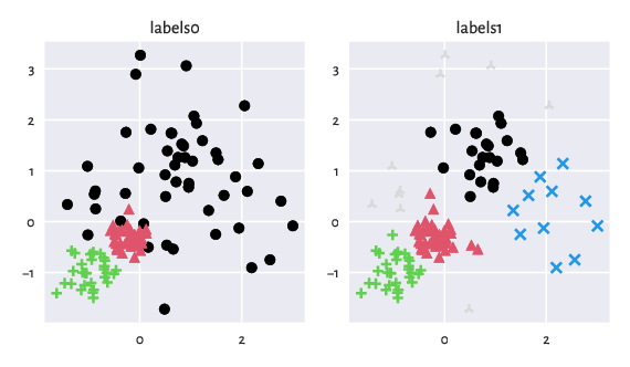
Figure 7: An example benchmark dataset and the corresponding ground truth labels.

Fetching Precomputed Results

Let us study one of the sets of precomputed clustering results stored in the following directory:

results_path = os.path.join("~", "Projects", "clustering-results-v1", "original")

They can be fetched by calling:

method_group = "Genie"  # or "*" for everything
res = clustbench.load_results(
    method_group, b.battery, b.dataset, b.n_clusters, path=results_path
)
print(list(res.keys()))
## ['Genie_G0.1', 'Genie_G0.3', 'Genie_G0.5', 'Genie_G0.7', 'Genie_G1.0']

We thus have got access to precomputed data generated by the Genie algorithm with different gini_threshold parameter settings.

Computing External Cluster Validity Measures

Different external cluster validity measures can be computed by calling clustbench.get_score:

pd.Series({  # for aesthetics
    method: clustbench.get_score(b.labels, res[method])
    for method in res.keys()
})
## Genie_G0.1    0.870000
## Genie_G0.3    0.870000
## Genie_G0.5    0.590909
## Genie_G0.7    0.666667
## Genie_G1.0    0.010000
## dtype: float64

By default, normalised clustering accuracy is applied. As explained in the tutorial, we compare the predicted clusterings against all the reference partitions (ignoring noise points) and report the maximal score.

Let us depict the results for the "Genie_G0.3" method:

method = "Genie_G0.3"
for i, k in enumerate(res[method].keys()):
    plt.subplot(1, len(res[method]), i+1)
    genieclust.plots.plot_scatter(
        b.data, labels=res[method][k]-1, axis="equal", title=f"{method}; k={k}"
    )
plt.show()

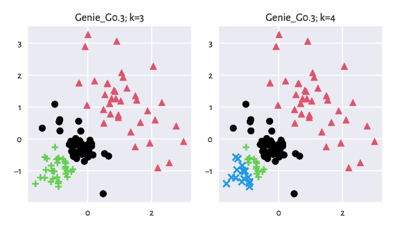
Figure 8: Results generated by Genie.

Applying Clustering Methods Manually

Naturally, the aim of this benchmark framework is also to test new methods. We can use clustbench.fit_predict_many to generate all the partitions required to compare ourselves against the reference labels.

For instance, let us investigate the behaviour of the k-means algorithm:

import sklearn.cluster
m = sklearn.cluster.KMeans(n_init=10)
res["KMeans"] = clustbench.fit_predict_many(m, b.data, b.n_clusters)
clustbench.get_score(b.labels, res["KMeans"])
## 0.9848484848484849

We see that k-means (which specialises in detecting symmetric Gaussian-like blobs) performs better than Genie on this particular dataset.

method = "KMeans"
for i, k in enumerate(res[method].keys()):
    plt.subplot(1, len(res[method]), i+1)
    genieclust.plots.plot_scatter(
        b.data, labels=res[method][k]-1, axis="equal", title=f"{method}; k={k}"
    )
plt.show()

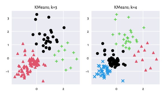
Figure 9: Results generated by K-Means.

For more functions, please refer to the package’s documentation (in the next section). Moreover, Colouriser: A Planar Data Editor describes a standalone application that can be used to prepare our own two-dimensional datasets.

Note that you do not have to use the clustering-benchmark package to access the benchmark datasets from our repository. The Access from Python, R, MATLAB, etc. section mentions that most operations involve simple operations on files and directories which you can implement manually. The package was developed merely for the users’ convenience.