True vs Predicted Clusters

Data

Let $X=\{{\mathbf{x}}_1,\dots ,{\mathbf{x}}_n\}$ be a benchmark dataset that consists of $n$ objects.

As an illustration, in this section, we consider the wut/x2 dataset, which features 120 points in ${\mathbb{R}}^2$.

import clustbench
data_url = "https://github.com/gagolews/clustering-data-v1/raw/v1.1.0"
benchmark = clustbench.load_dataset("wut", "x2", url=data_url)
X = benchmark.data
X[:5, :]  # preview
## array([[-0.16911746, -0.25135197],
##        [-0.17667309, -0.48302249],
##        [-0.1423283 , -0.36194485],
##        [-0.10637601, -0.70068834],
##        [-0.49353012, -0.23587515]])

Note

Python code we give here should be self-explanatory even to the readers who do not know this language (yet[1]). Also note that in a further section, we explain how to use our benchmark framework from within R and MATLAB.

Reference Labels

Each benchmark dataset is equipped with a reference[2] partition assigned by experts, which represents a grouping of the points into $k\ge 2$ clusters, or, more formally, a k-partition[3] $\{X_1,\dots ,X_k\}$ of $X$.

(y_true := benchmark.labels[0])  # the first label vector
## array([2, 2, 2, 2, 2, 2, 2, 2, 2, 2, 2, 2, 2, 2, 2, 2, 2, 2, 2, 2, 2, 2,
##        2, 2, 2, 2, 2, 2, 2, 2, 2, 2, 2, 2, 2, 2, 2, 2, 2, 2, 1, 1, 1, 1,
##        1, 1, 1, 1, 1, 1, 1, 1, 1, 1, 1, 1, 1, 1, 1, 1, 1, 1, 1, 1, 1, 1,
##        1, 1, 1, 1, 1, 1, 1, 1, 1, 1, 1, 1, 1, 1, 1, 1, 1, 1, 1, 1, 1, 1,
##        1, 1, 3, 3, 3, 3, 3, 3, 3, 3, 3, 3, 3, 3, 3, 3, 3, 3, 3, 3, 3, 3,
##        3, 3, 3, 3, 3, 3, 3, 3, 3, 3])

More precisely, what we have here is a label vector $\mathbf{y}$, where $y_i\in \{1,\dots ,k\}$ gives the subset/cluster number (ID) of the i-th object.

The number of subsets, k, is thus an inherent part of the reference set:

(k := max(y_true))  # or benchmark.n_clusters[0]
## np.int64(3)

Predicted Labels

Let us take any partitional clustering algorithm whose quality we would like to assess. As an example, we will consider the outputs generated by Genie. We apply it on $X$ to discover a new k-partition:

import genieclust
g = genieclust.Genie(n_clusters=k)  # using default parameters
(y_pred := g.fit_predict(X) + 1)  # +1 makes cluster IDs in 1..k, not 0..(k-1)
## array([1, 1, 1, 1, 1, 1, 1, 1, 1, 1, 1, 1, 1, 1, 1, 1, 1, 1, 1, 1, 1, 1,
##        1, 1, 1, 1, 1, 1, 1, 1, 1, 1, 1, 1, 1, 1, 1, 1, 1, 1, 1, 1, 2, 1,
##        2, 2, 2, 2, 2, 2, 2, 2, 1, 2, 2, 2, 1, 1, 2, 3, 2, 2, 2, 2, 2, 1,
##        2, 2, 2, 2, 2, 1, 2, 2, 2, 2, 2, 1, 2, 2, 2, 1, 2, 1, 2, 2, 2, 2,
##        2, 1, 3, 3, 3, 3, 3, 3, 3, 3, 3, 3, 3, 3, 3, 3, 3, 3, 3, 3, 3, 3,
##        3, 3, 3, 3, 3, 3, 3, 3, 3, 3])

We thus obtained a vector of predicted labels encoding a new grouping, $\{{\hat{X}}_1,\dots ,{\hat{X}}_k\}$. We will denote it by $\hat{\mathbf{y}}$.

The figure below depicts the two partitions side by side.

plt.subplot(1, 2, 1)
genieclust.plots.plot_scatter(X, labels=y_true-1, axis="equal", title="y_true")
plt.subplot(1, 2, 2)
genieclust.plots.plot_scatter(X, labels=y_pred-1, axis="equal", title="y_pred")
plt.show()

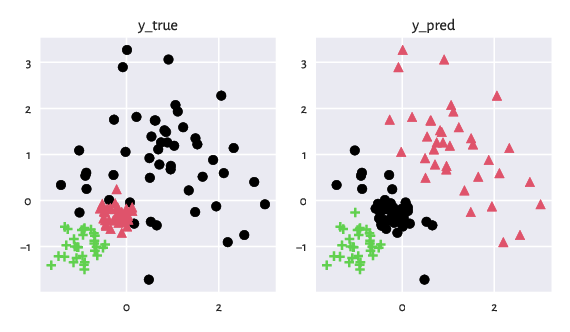
Figure 1: Two example partitions that we would like to compare. Intuitively, clustering can be considered as a method to assign colours to all the input points.

Important

Ideally, we would like to work with algorithms that yield partitions closely matching the reference ones. This should be true on as wide a set of problems as possible.

We, therefore, need to relate the predicted labels to the reference ones. Note that the automated discovery of $\hat{\mathbf{y}}$ never relies on the information included in $\mathbf{y}$ (except for the cluster count, $k$). In other words, clustering is an unsupervised[4] learning process.

Permuting Cluster IDs

A partition is a set of point groups, and sets are, by definition, unordered. Therefore, the actual cluster IDs do not matter. Looking at the above figure, we see that the red (ID=2), black (ID=1), and green (ID=3) predicted clusters can be paired with, respectively, the black (ID=1), red (ID=2), and green (ID=3) reference ones. We can easily recode[5] y_pred so that the cluster IDs correspond to each other:

import numpy as np
o = np.array([2, 1, 3])  # relabelling: 1→2, 2→1, 3→3
(y_pred := o[y_pred-1])  # Python uses 0-based indexing, hence the -1
## array([2, 2, 2, 2, 2, 2, 2, 2, 2, 2, 2, 2, 2, 2, 2, 2, 2, 2, 2, 2, 2, 2,
##        2, 2, 2, 2, 2, 2, 2, 2, 2, 2, 2, 2, 2, 2, 2, 2, 2, 2, 2, 2, 1, 2,
##        1, 1, 1, 1, 1, 1, 1, 1, 2, 1, 1, 1, 2, 2, 1, 3, 1, 1, 1, 1, 1, 2,
##        1, 1, 1, 1, 1, 2, 1, 1, 1, 1, 1, 2, 1, 1, 1, 2, 1, 2, 1, 1, 1, 1,
##        1, 2, 3, 3, 3, 3, 3, 3, 3, 3, 3, 3, 3, 3, 3, 3, 3, 3, 3, 3, 3, 3,
##        3, 3, 3, 3, 3, 3, 3, 3, 3, 3])

See below for an updated figure.

plt.subplot(1, 2, 1)
genieclust.plots.plot_scatter(X, labels=y_true-1, axis="equal", title="y_true")
plt.subplot(1, 2, 2)
genieclust.plots.plot_scatter(X, labels=y_pred-1, axis="equal", title="y_pred")
plt.show()

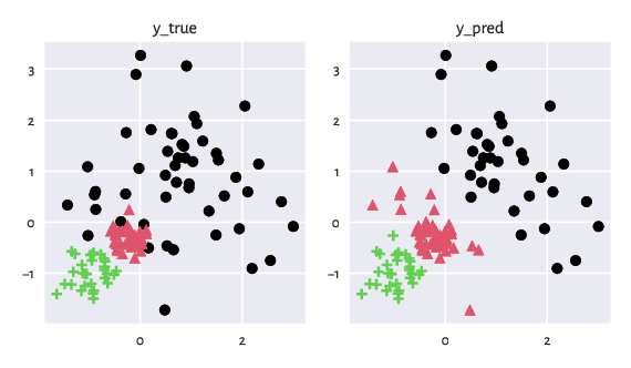
Figure 2: The two partitions after the cluster ID (colour) matching.

Confusion Matrix

We can determine the confusion matrix $\mathbf{C}$ for the two label vectors:

genieclust.compare_partitions.confusion_matrix(y_true, y_pred)
## array([[37, 12,  1],
##        [ 0, 40,  0],
##        [ 0,  0, 30]])

Here, the value in the $i$-th row and the $j$-to column, $c_{i,j}$, denotes the number of points in the $i$-th reference cluster that the algorithm assigned to the $j$-th cluster.

Overall, Genie returned a clustering quite similar to the reference one. We may consider 107 (namely, $c_{1,1}+c_{2,2}+c_{3,3}=37+40+30$) out of the 120 input points as correctly grouped. In particular, all the red and green reference points (the 2nd and the 3rd row) have been properly discovered.

However, the algorithm has miscategorised (at least, as far as the current set of expert labels is concerned) one green and twelve red points. They should have been coloured black.

External Cluster Validity Measures

A confusion matrix summarises all the information required to judge the similarity between the two partitions. However, if we wish to compare the quality of different algorithms, we would rather have it summarised in the form of a single number.

Following [24], we recommend the use of the normalised clustering accuracy (NCA) as an external cluster validity measure which quantifies the degree of agreement between the reference $\mathbf{y}$ and the predicted $\hat{\mathbf{y}}$. It is given by:

$$\mathrm{NCA}(\mathbf{C})={\displaystyle \underset{\sigma :\{1,\dots ,k\}\stackrel{\text{1--1}}{\to }\{1,\dots ,k\}}{max}\frac{1}{k}{\displaystyle \sum _{j=1}^k\frac{c_{\sigma (j),j}-\frac{1}{k}{c}_{\sigma (j),j}}{c_{\sigma (j),\cdot }-\frac{1}{k}{c}_{\sigma (j),\cdot }}.}}$$

NCA is the averaged percentage of correctly classified points in each cluster above the perfectly uniform label distribution. Note that the matching between the cluster labels is performed automatically by finding the best permutation $\sigma$ of the set $\{1,\dots ,k\}$.

Overall, the more similar the partitions, the greater the similarity score. Two identical clusterings yield the value of 1. NCA is normalised: it is equal to 0 if the cluster memberships are evenly spread or all the points were put into a single large cluster. In our case:

genieclust.compare_partitions.normalized_clustering_accuracy(y_true, y_pred)
## 0.8700000000000001

or, equivalently:

clustbench.get_score(y_true, y_pred)  # the NCA metric is used by default
## np.float64(0.8700000000000001)

This value indicates a decent degree of similarity between the reference and the discovered partitions.

Other popular partition similarity scores, e.g., the adjusted Rand index or normalised mutual information, are discussed in the Appendix. In particular, this is where we argue why the classic (classification) accuracy rate should not be used in our context (a common mistake!).

---

[1]

Check out Marek’s open-access (free!) textbook Minimalist Data Wrangling in Python [23].

[2]

Later we will note that there may be many equally valid ways to split a dataset into groups.

[3]

We say that $\{X_1,\dots ,X_k\}$ is a $k$-partition of $X$, whenever $\bigcup _{i=1}^k{X}_i=X$, each $X_i$ is nonempty, and the subsets are pairwise disjoint, i.e., $X_i\cap X_j=\mathrm{\varnothing }$ for $i\ne j$.

[4]

Tasks such as semi-supervised clustering, where the right assignment of some of the input points is known in advance, are not of our interest here. However, the current framework can trivially be adjusted to fit such scenarios.

[5]

In a later section, we discuss a way to automatically discover an optimal relabelling based on the solution to the maximal assignment problem.