Noise Points¶

To make the clustering task more challenging, some benchmark datasets feature noise points (e.g., outliers or irrelevant points in-between the actual clusters). They are specially marked in the ground-truth vectors: we assign them cluster IDs of 0.

Example¶

Let us consider the other/hdbscan dataset [40], which consists of 2,309 points in \(\mathbb{R}^2\).

import numpy as np
import pandas as pd
import clustbench
# Accessing <https://github.com/gagolews/clustering-data-v1> directly:
data_url = "https://github.com/gagolews/clustering-data-v1/raw/v1.1.0"
benchmark = clustbench.load_dataset("other", "hdbscan", url=data_url)
X = benchmark.data
y_true = benchmark.labels[0]

Here is a summary of the number of points in each reference cluster:

pd.Series(y_true).value_counts()
## 0    510
## 1    410
## 2    366
## 3    326
## 4    306
## 5    207
## 6    184
## Name: count, dtype: int64

There are six clusters (1–6) and a special point group with ID=0 that marks some points as noise.

import genieclust
genieclust.plots.plot_scatter(X, labels=y_true-1, axis="equal", title="y_true")
plt.show()

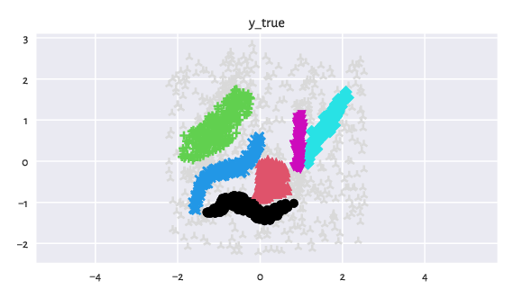
../_images/partition-similarity-noise-data-1.png — Figure 3: An example dataset featuring noise points (light grey whatchamacallits).¶

Discovering Clusters¶

Suppose we want to evaluate how Genie handles such a noisy dataset.

Important

The algorithm must not be informed about the exact location of the noise points. After all, it is an unsupervised learning task.

k = np.max(y_true)  # the number of clusters to detect
g = genieclust.Genie(n_clusters=k)  # using default parameters
y_pred = g.fit_predict(X) + 1  # +1 makes cluster IDs in 1..k, not 0..(k-1)

Below we plot the predicted partition. Additionally, we draw its version where the noise point markers are propagated from the ground truth vector (as a kind of data postprocessing).

plt.subplot(1, 2, 1)
genieclust.plots.plot_scatter(X, labels=y_pred-1, axis="equal", title="y_pred")
plt.subplot(1, 2, 2)
y_pred2 = np.where(y_true > 0, y_pred, 0)  # y_pred, but noise points get ID=0
genieclust.plots.plot_scatter(X, labels=y_pred2-1, axis="equal",
    title="y_pred (noise from y_true)")
plt.show()

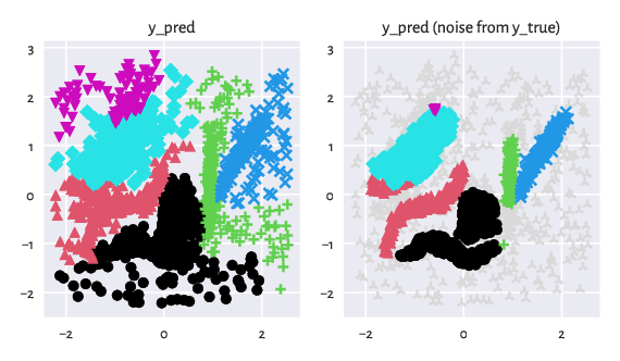
../_images/partition-similarity-noise-genie-3.png — Figure 4: Noise points make the life of a clustering algorithm harder.¶

Evaluating Similarity¶

Here is the confusion matrix:

genieclust.compare_partitions.confusion_matrix(y_true, y_pred)
## array([[116,  84, 124,  51,  52,  83],
##        [409,   0,   1,   0,   0,   0],
##        [366,   0,   0,   0,   0,   0],
##        [  0,  24,   0,   0, 298,   4],
##        [  0, 306,   0,   0,   0,   0],
##        [  0,   0,   0, 207,   0,   0],
##        [  0,   0, 184,   0,   0,   0]])

The first row denotes the “noise cluster”.

Genie recreated four of the reference clusters very well (3, 4, 5, 6), but failed on the first two (it discovered a “combined” cluster instead, and considered some noise points as a separate set).

Important

When computing external cluster validity measures, we should omit the noise points from the reference set whatsoever. After all, most classical algorithms are not equipped with noise point detectors[1] and they should not be penalised for this.

Let us compute the normalised clustering accuracy, ignoring the first row in the confusion matrix:

genieclust.compare_partitions.normalized_clustering_accuracy(
    y_true[y_true>0],
    y_pred[y_true>0]
)
## 0.7828220858895705

or, equivalently:

clustbench.get_score(y_true, y_pred)  # the NCA metric is used by default
## 0.7828220858895705

The score is somewhere between 4/6 (four clusters discovered correctly) and 5/6 (one cluster definitely missed).